arb multiphysics finite volume solver
New version 0.60 uploaded (9/4/19) that includes some extended vector/tensor capabilities.
What is arb?
arb is a software package designed to solve arbitrary partial differential equations on unstructured meshes using an implicit finite volume method. The primary strengths of arb are:
- All equations and variables are defined using 'maths-type' expressions written by the user, and hence can be easily tailored to each application;
- All equations are solved simultaneously using a Newton-Raphson method, so implicitly discretised equations can be solved efficiently; and
- The unstructured mesh over which the equations are solved can be composed of all sorts of convex polygons/polyhedrons. One, two and three dimensional domains can be used (simultaneously).
arb is open-source software that is released under the GNU General Public Licence (GPL). arb was originally created by Dalton Harvie, but is now a collaborative project.
Some examples
A diffusion problem:
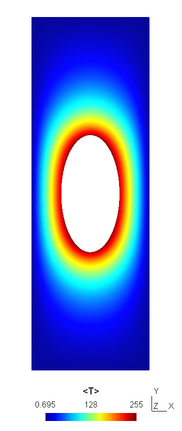
The image (right) shows the solution to the following diffusion problem solved over a 2D domain:

This set of equations is represented by the following in arb:
CELL_EQUATION <T transport>
"-celldiv(<D>*facegrad(<T>))" ON <domain>
FACE_EQUATION <T hole>
"-<D>*facegrad(<T>)-<hole flux>" ON <hole>
FACE_EQUATION <T walls> "<T>-1.0d0" ON <walls>
Four main variables are defined in this example: the unknown temperature field (with optional units Kelvin), and three equation variables. Each variable is associated with a region. The temperature (<T>) is defined over all cells (<allcells>), while the equations are specific to either all of the domain cells (<domain>) or as boundary conditions on particular boundary (face) regions (<hole> and <walls>). The equations are satisfied when the equation variable values are zero: Within arb the Newton-Raphson method is used to change the unknown variable values until this is achieved. Hence the core constraint in an arb simulation is that the total number of unknown variable values equals the total number of equation values. In this particular example this is satisfied as the number of elements within the <allcells> region equals the sum of elements within the <domain>, <hole> and <walls> regions.
Other variable types include DERIVED, CONSTANT, TRANSIENT, NEWTIENT, LOCAL, OUTPUT and CONDITION. Other variable centrings are NODE and NONE. Variables can also be identified as a component of a vector (eg <u[l=1]>) or tensor (eg <tau[l=2,3]>). They can also associated with a particular relative timestep for transient simulations (eg <t[r=1]> representing the time at the previous timestep).
Operators are used to express equations using the finite volume method: For example, celldiv performs a divergence around a cell element while facegrad calculates the gradient of a quantity relative to a face element. Other operators allow sums to be performed over regions (eg cellsum), linking between different regions and computational domains (eg facetocelllink) and conditional statements (eg nodeif). Some elementary vector algebra is also implemented (eg dot and double dot products).
This problem is included with the arb distribution as tutorial 1. You can browse the arb input file here. Note that anything following a '#' symbol is a comment.
Steady-state flow around a cylinder:
The two-dimensional flow around a cylinder is a CFD benchmark test problem. Here the Reynolds number based on the cylinder diameter and maximum velocity is 20, producing steady-state results.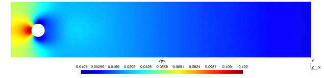
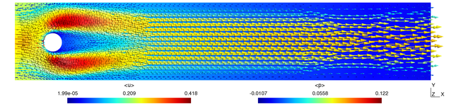
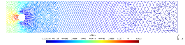
This problem is also included with the arb distribution as tutorial 3. You can browse the arb input file here.
Other problems:
Many more example problems are included as input and geometry files with the arb distribution. Browsing these is at present the best way to learn the syntax and understand the capabilities of arb. Examples include transient problems, multi-dimensional (0D-3D) problems, systems of ODEs (eg, multi-component chemical equations) and multiphase (eg, Volume of Fluid) flows. You can find these files here.
Manual:
An online manual is under development here.
What is needed to run arb?
In terms of coding content arb consists mainly of fortran (2003), perl and shell scripts. arb requires a UNIX type environment to run, and is maintained on both the Apple OsX and ubuntu linux platforms. We have also used it on Red-Hat linux and Windows Subsystem for Linux (WSL).
arb depends on certain third party programs and libraries, including:
- A fortran compiler; the Intel compiler ifort or GNU compiler gfortran;
- The computer algebra system maxima;
- A sparse matrix linear solver: UMFPACK, pardiso (both the native and ifort versions) or a Harwell Subroutine Library routine; and
- The mesh generation and post-processing package gmsh.
By combining gfortran with the UMFPACK sparse linear solver, arb can be run using freely available GPL licensed software.
Try it out
Getting up and running is relatively straightforward, and primarily consists of installing the software and packages on which arb depends.
Download the arb code
Firstly you need to download the arb code working directory and place it somewhere where it can stay. A tar file containing the latest master arb source is here. Older versions can be found in this directory. Alternatively you can grab the install files from github. These versions haven't been updated for a while for licencing reasons, so contact me if you want a more recent version.
Install dependencies
On recent versions of ubuntu (tested on LTS 10.04, 12.04, 14.04, 16.04, 18.04 and 20.04) you can run the ubuntu install script (found in the install directory) which will use apt-get to install the required packages. This doesn't take long. There is also an install script for red hat in the same directory, although this is not as well tested.
If you want to install arb on Windows, this is now possible using the Windows Subsystem for Linux (WSL) on Windows 10. WSL basically installs a recent ubuntu version within a user's directory. Once you have this working (you'll have to find instructions on how to do this) then just follow the ubuntu arb install instructions. WSL is actually quite easy.
Installation on OsX is usually straightforward, being based on macports (which needs to be installed first). However, macports generally compiles software, so it will take some time to install all the dependencies from scratch (maybe an hour?). The install script for OsX is the macports install script also in the install directory.
Add arb to your path
For all platforms, once the code is downloaded and the dependencies are installed then run the install_globally.sh script (also in the install directory) to place the executables in your path. Then restart your terminal, and you should be ready to start simulating. Try tutorial problem 1 from the examples directory to check that all is working fine. More details about this problem are given in the second screencast below
Screencasts
The following screencast deals with installing arb and running a trial simulation. Unfortunately this first screencast was produced using v0.56 which required a separate arb working directory for each simulation. From v0.57 and onwards arb is installed globally, so there will be slight differences in the arb directory structure and installation method (refer to the above scripts for installation).
This next monster screencast covers the basics of arb use, including the arb directory structure, altering mesh files and basic arb coding. Again note that this screencast was produced using v0.56, in which simulations were conducted in separate arb working directories. Most of the content is still relevant however.
Contribute
To actively contribute to this project, email Dalton for a username on our gitlab development server. Feel like writing some documentation? Don't hold back.
Citing
If you use arb to conduct research, please cite it using the publication (Dalton J.E. Harvie, ANZIAM J. 52, 2012) given below. I am keen to hear of your experiences using arb and also of any feature requests that you have and bugs that you find - drop me an email with 'arb' in the subject line.
Where is arb going?
arb is under active development, although updates to this website have sometimes not occurred regularly. Previously the major focus was on developing the language feature set - application of arb to different types of problems (in particular multiphase and non-Newtonian flows) is now the development focus, as well as improving installation ease and overall documentation. At some stage I will be organising a few hour familiarisation session - drop me an email if you are interested in attending this.